In this post, I am trying to understand the reason why LSTM can deal with vanishing and exploding gradient so that it is better than normal RNN in modeling long-term dependencies in sequential data. To start with, we have to comprehend what are vanishing and exploding gradient. Paper [1] is a really good reference to this.

Basically, back propagation is the fundamental method used to train a neural network. In recurrent neural networks (or deep neural networks), due to the reason that the gradient has to propagate back multiple time step, it is running the risk that the gradient will reduce to 0 or explode to a huge number.

1.Vanishing and Exploding Gradient

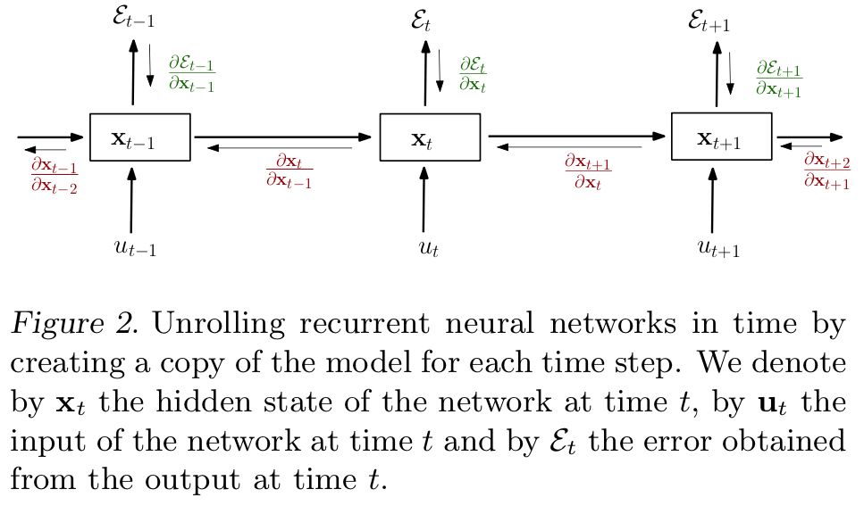
More formally, as shown in Fig.2 (cited from [1]), to perform gradient descent, one has to compute the gradients for the parameters inside the hidden unit. Due to the reason that the hidden unit is shared along all the time steps, the gradients for the parameters inside the hidden unit could be concluded as:

$\frac{\partial \varepsilon}{\partial \theta} = \sum_{1\leq t\leq T} \frac{\partial \varepsilon_t}{\partial \theta}$ ,

where $\varepsilon_t$ is the error measure (loss) in time $t$ , and $\varepsilon$ is the group of all error measures from time 1 to $t$ . While, $\theta$ is the vector of parameters in the shared hidden unit. Thus, the formula above aggregates the information given by all the error measures in each time step to identify the overall gradient for updating the parameters. Afterward, for each time step, the partial derivative could be further decomposed as:

$\frac{\partial \varepsilon_t}{\partial \theta} = \sum_{1\leq k \leq t} \Big( \frac{\partial \varepsilon_t}{\partial x_t}\frac{\partial x_t}{\partial x_k}\frac{\partial x_k}{\partial \theta} \Big)$ .

Furthermore, we can find that:

$\frac{\partial x_t}{\partial x_k} = \prod_{k < i \leq t} \frac{\partial x_i}{\partial x_{i-1}}$ .

Then here comes the question. When $\frac{\partial x_i}{\partial x_{i-1}}$ is always smaller than a constant $\eta < 1$ , it has the product of gradients goes to 0 exponentially fast with $t - k$ :

$\frac{\partial x_t}{\partial x_k} = \prod_{k < i \leq t} \frac{\partial x_i}{\partial x_{i-1}} \leq \eta^{t-k} < 1$ .

Similarly, if the value of the derivative is always greater than 1 or bigger, it is running the risk of gradient explosion, i.e., the gradient increases exponentially. Note that we are using one-dimensional case here to illustrate the problem. Please refer to [1] for multi-dimensional case.

2.Why LSTM Works?

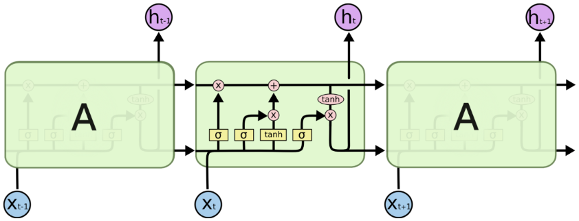
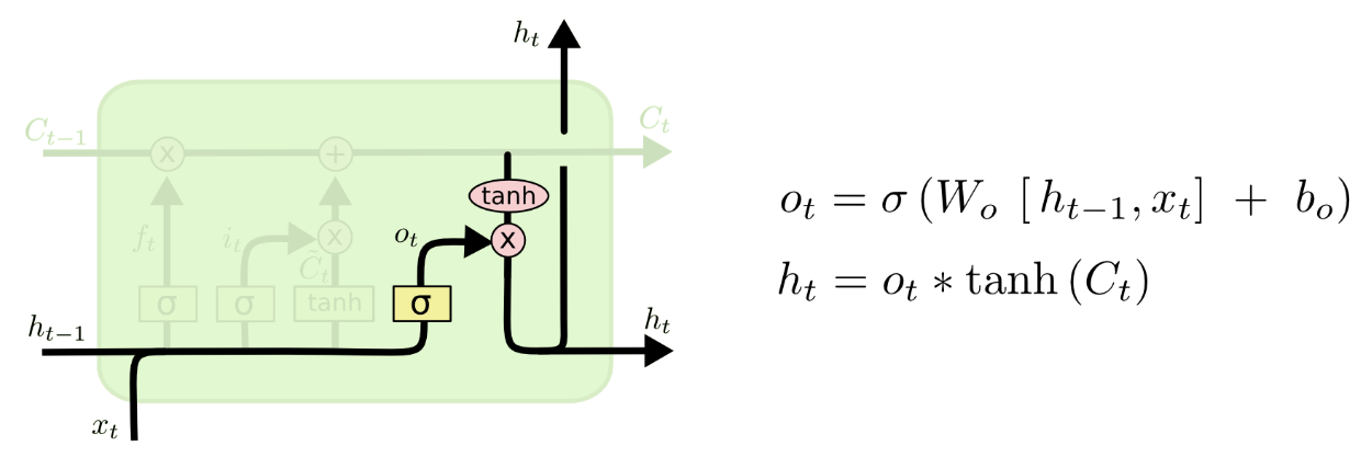
It is now clear that the key to ease the issue of vanishing and exploding gradient is to carefully manipulate the partial derivative $\frac{\partial x_i}{\partial x_{i-1}}$ to maintain a reasonable value of the overall gradient $\frac{\partial \varepsilon}{\partial \theta}$ .

In the figure above (quoted from Colah’s blog), it shows the inner structure of a LSTM unit. The input/output is composed of two parts: a context state and a hidden state (shown below, quoted from Colah’s blog). Sorry for the abuse of notation $x$ here. In the figures, $x$ is the input for a LSTM unit, while in the previous section, we use $x$ as the hidden state in a RNN cell.

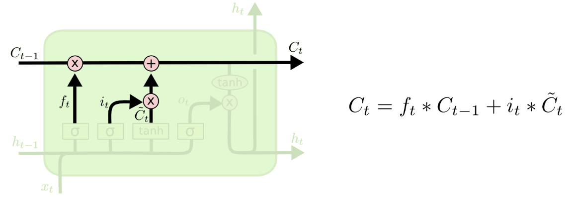
It can be derived from previous section that $\frac{\partial h_t}{\partial h_{t-k}}$ is still the product of a series of derivatives. We could put it more formally and derive that:

$\frac{\partial h_t}{\partial h_{t-k}} = \prod_{1 < i \leq t} \frac{\partial h_i}{\partial h_{i-1}} = \prod_{1 < i \leq t} \Big(\frac{\partial h_i}{\partial C_i}\frac{\partial C_i}{\partial h_{i-1}} + \frac{\partial h_i}{\partial o_i}\frac{\partial o_i}{\partial h_{i-1}} \Big)$ .

This is due to the reason that in each LSTM cell, there are two paths that $h_{i-1}$ could affect $h_{i}$ .

More importantly, it is noticed that, after solving the product, we could find an item:

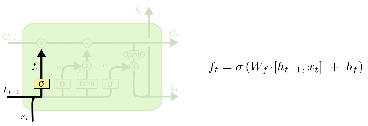
$\frac{\partial h_t}{\partial C_t}\frac{\partial C_t}{\partial h_{t-1}}\frac{\partial h_{t-1}}{\partial C_{t-1}}\frac{\partial C_{t-1}}{\partial h_{t-2}} \cdots \frac{\partial h_{t-k+1}}{\partial C_{t-k+1}}\frac{\partial C_{t-k+1}}{\partial h_{t-k}} = \frac{\partial h_t}{\partial C_t}\frac{\partial C_t}{\partial C_{t-1}} \cdots \frac{\partial C_{t-k+2}}{\partial C_{t-k+1}}\frac{\partial C_{t-k+1}}{\partial h_{t-k}}$

$= \frac{\partial h_t}{\partial C_t} \frac{\partial C_{t-k+1}}{\partial h_{t-k}} \prod_{0<i\leq k-2} \frac{\partial C_{t-i}}{\partial C_{t-i-1}}$ ,

in which the product can be further analysed as (notations could be found in following figure, quoted from Colah’s blog):

$\prod_{0<i\leq k-2} \frac{\partial C_{t-i}}{\partial C_{t-i-1}} = \prod_{t-k+2 < i < t} f_i = \prod_{t-k+2 < i < t} \sigma (W_i[h_{i-1}, x_i]+b_i)$

It is discussed in thesis [2] (page 14) that the quantity of this product is safe from vanishing and exploding. Therefore, we are optimistic that the overall gradient, i.e., $\frac{\partial \varepsilon }{\partial \theta}$ , will not be too small or too big so that same from vanishing and exploding gradient. Note here again that:

$\frac{\partial \varepsilon }{\partial \theta} = \sum_{1\leq t \leq T} \frac{\partial \varepsilon_t}{\partial \theta} = \sum_{1\leq t \leq T}\sum_{1\leq k \leq t} \frac{\partial \varepsilon_t}{\partial h_t}\frac{\partial h_t}{\partial h_{t-k}}\frac{\partial h_{t-k}}{\partial \theta}$ .

3.Discussion

To be honest, I am not fully convinced by the aforementioned derivation. The key product can certainly approach 0 in specifica cases, although it will not explode. Hence, I am still waiting for better explanation. Practical experiments have shown that LSTM can be trained but it still has limitations in extracting long-term patterns/dependencies of sequential data. Certain research has tried to supersede the utilisation of RNN with other mechanism, e.g., Attention is all you need. Maybe, I mean maybe, RNN is not really necessary?

4.References

[1] Razvan Pascanu, Tomas Mikolov, Yoshua Bengio, On the difficulty of training recurrent neural networks, ICML, vol. 3, no. 28, pp. 1310-1318, 2013.

[2] Justin Simon Bayer, Learning Sequence Representations, Dissertation, Technische Universität München, 2015.

[3] quora.com question

[4] stackexchange.com question